
The Euler-Lagrange equation stands as a core differential equation within the calculus of variations, serving to pinpoint the function where a specified functional attains an extremal value. It furnishes the requisite criterion for an optimum, like a lowest point or highest point, through the connection of a scalar function’s partial rate of changes to its complete rate of change across time or area.
Foundations of the Calculus of Variation
The Calculus of variation deals with determining the curve or area that either lessens or enlarges a designated value, called a functional. Contrasting with conventional calculus, which locates extreme points of functions, this discipline identifies whole functions yielding stationary results. You use this mathematical framework to solve problems like the shortest distance between two points or the path of quickest descent for a falling object.
In theRPSC Assistant Professor Maths Syllabus, the calculus of variations forms a cornerstone for grasping physical mechanisms and optimizing shapes. The alteration of a functional entails scrutinizing how slight variations in the function impact the resulting integral amount. This procedure directly yields the Euler-Lagrange equation. Proficiency in this area enables tackling boundary condition assignments in both ordinary and partial differential equations. Applicants studying former RPSC Assistant Professor Maths (PYQs) frequently observe these fundamentals when determining the shortest paths or surfaces with the least area.
Deriving the Euler-Lagrange Equation for Functional Variation
The Euler-Lagrange equation stems from the condition that the initial change in a functional must be zero. Take a functional J[y] expressed as the integral of a function F(x, y, y’). Determining the function y(x) that optimizes J[y] necessitates fulfilling a particular second-order standard differential equation. This equation serves as the connection linking the integrated form to the local characteristics of the best-suited path.
The numerical expression of the Euler-Lagrange equation is given by:
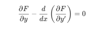
In this expression, y’ represents the first derivative of $y$ with respect to x. When you apply this to the RPSC Assistant Professor Maths Syllabus, you solve for y by integrating the resulting differential equation. This formula remains the primary tool for identifying the variation of a functional in physics and engineering. VedPrep students often use this expression to simplify complex mechanics problems into solvable differential forms.
Necessary and Sufficient Conditions for Extrema
The Euler-Lagrange expression offers a prerequisite for an extremum; thus, any function that minimizes or maximizes must adhere to it. Nevertheless, meeting this equation’s requirements does not assure the outcome is a minimum or a maximum. Additional assessments, like examining the second variation or Legendre criteria, are needed to ascertain if the stationary point represents a genuine extremum. This difference is crucial when reviewing the RPSC Assistant Professor Maths (PYQs), as numerous problems demand demonstration of the stationary curve’s character.
A sufficient condition often involves the Jacobi condition or the Weierstrass excess function. These advanced checks ensure that the path found via the Euler-Lagrange equation is stable against all possible small variations. Within the field of variational calculus, a function meeting the required criteria is termed an extremal. Educators at VedPrep stress that although the Euler-Lagrange equation points to potential answers, only the sufficient conditions verify the physical validity of the result.
Variational Methods for Boundary Value Problems
Transforming differential equation boundary value problems, ordinary and partial, into optimization exercises is the role of variational methods. Rather than tackling the equation head-on, one seeks a function that yields the lowest value for an associated energy functional. This technique proves highly useful for partial differential equations where straightforward integration proves challenging. These methods are featured in the RPSC Assistant Professor Maths Syllabus as they underpin finite element techniques and computational simulation.
By specifying the change in a functional across a chosen range with constant limits, one can obtain the fundamental equations describing the system. This technique is relevant to areas like thermal transfer, material deformation, and quantum theory. Reviewing RPSC Assistant Professor Maths (PYQs) reveals that numerous boundary condition problems are structured around locating the maximum or minimum value of an integrated action. This single viewpoint streamlines the examination of various mathematical and physical frameworks.
Core Theorems and Formulas
The following table summarizes the key theorems and mathematical forms related to the Euler-Lagrange equation within the calculus of variation.
| Theorem Name | Mathematical Form / Condition | Application Context |
|---|---|---|
| Standard Euler-Lagrange | 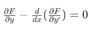 |
Single independent variable optimization |
| Beltrami Identity | 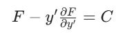 |
Used when $F$ does not explicitly depend on x |
| Legendre Condition | 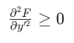 |
Necessary condition for a local minimum |
| Ostrogradsky Equation | 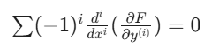 |
Functionals with higher order derivatives |
Limitations and Critical Perspectives on Variational Solutions
A frequent misstep when utilizing the Euler-Lagrange equation is the presumption that it invariably produces a sleek, unbroken result. In practice, certain functionals lack a well-behaved peak or trough within the set of continuous mappings. This arises if the function being integrated lacks sufficient regularity, or if the specified limits necessitate a sharp discontinuity. Consequently, the solution derived from the Euler-Lagrange equation might fail to honor the initial restrictions of the physical scenario.
To lessen these constraints, confirm the solution’s presence prior to trying to resolve the differential equation. For intricate situations involving PDEs, a functional’s variation could yield several equilibrium trajectories. Always examine the physical restrictions, like positiveness or energy constancy, in order to pinpoint the right solution branch. This methodical accuracy distinguishes high achievers in the RPSC Assistant Professor Maths examination from those merely using formulas without deeper thought.
Practical Application: The Brachistochrone Problem
The Brachistochrone challenge is a well-known use of the calculus of variations. The aim is to determine the curve of a flexible cable upon which a small particle moves solely due to gravity, spanning between two fixed locations, arriving in the minimum possible duration. By formulating the travel duration as a functional, one employs the Euler-Lagrange equation to uncover the ideal trajectory. The solution is a cycloid, rather than a direct line, illustrating that the shortest route is not invariably the quickest.
This situation underscores the significance of the RPSC Assistant Professor Maths Syllabus in grasping how the world actually functions. By quantifying the change in a functional, one ascertains the interplay between gravity and the shape of space in affecting movement. VedPrep furnishes comprehensive answers to RPSC Assistant Professor Maths (Prior Year Questions) covering these practical uses, so you grasp both the underlying concepts and the process of applying variational methods.
Conclusion
Achieving command of the Euler-Lagrange equation marks a notable stage in your advancement through mathematics. This potent instrument offers a cohesive structure for tackling intricate challenges in physics, geometry, and engineering by pinpointing the inherent routes systems adopt. Although its derivation demands precise calculus, the skill to convert an integral functional into a solvable differential equation characterizes a proficient mathematician. As you proceed with the calculus of variations, recall that steady application across varied boundary constraints will sharpen your interpretive insight. VedPrep serves as your committed associate throughout this endeavor, furnishing the materials and skilled direction essential for success in the RPSC Assistant Professor examination.
To learn more in detail from our faculty, watch our YouTube video:
Frequently Asked Questions (FAQs)
How does the Euler-Lagrange equation relate to the calculus of variation?
Calculus of variation deals with finding functions that optimize a specific integral. The Euler-Lagrange equation serves as the primary tool to transform these integral problems into differential equations. It ensures that the first variation of the functional vanishes at the optimal path.
What is a functional in mathematics?
A functional is a mapping from a space of functions to the real numbers. In the RPSC Assistant Professor Maths Syllabus, functionals typically appear as integrals. The value of the functional depends on the entire shape of the input function rather than a single point.
Why is the Euler-Lagrange equation important for physics?
This equation forms the basis of Lagrangian mechanics. It allows physicists to derive the equations of motion for complex systems by minimizing the action functional. It represents the principle of least action, which governs the behavior of classical and quantum systems.
What defines an extremal in variational calculus?
An extremal is a function that satisfies the Euler-Lagrange equation. While every minimum or maximum is an extremal, not every extremal is a true extremum. You must verify sufficient conditions to confirm if the stationary point is a minimum, maximum, or saddle point.
How do you solve the Euler-Lagrange equation for a given problem?
First, identify the integrand F from the functional. Calculate the partial derivatives of F with respect to y and y'. Substitute these into the Euler-Lagrange formula and solve the resulting differential equation using boundary conditions. This process identifies the optimal path.
When should you use the Beltrami Identity?
Use the Beltrami Identity when the integrand F does not explicitly depend on the independent variable x. The identity simplifies to F - y'Fy' = C, where C is a constant. This reduces the second order equation to a first order equation, speeding up the solution.
How do you handle multiple dependent variables?
For functionals involving several functions like y(x) and z(x), you solve a system of simultaneous Euler-Lagrange equations. You generate one equation for each dependent variable. The set of solutions determines the optimal trajectory in multi dimensional space.
What are boundary conditions in variational problems?
Boundary conditions specify the values of the function y(x) at the start and end points of the interval. In the RPSC Assistant Professor Maths Syllabus, these conditions are essential to determine the constants of integration. Without them, you obtain a general family of curves.
What if the Euler-Lagrange equation has no solution?
A lack of solution often means the functional does not have a stationary point within the chosen class of functions. This happens if the integrand is not regular or if the boundary conditions are incompatible. You must re-examine the physical constraints or expand the function space.
Why does my extremal not yield a minimum value?
The Euler-Lagrange equation only identifies stationary points where the first variation is zero. It does not distinguish between minima and maxima. You must check the second variation or the Legendre condition to determine the nature of the stationary point.
How do you fix a singular Euler-Lagrange equation?
Singularities occur when the coefficient of the highest derivative vanishes. This often indicates that the functional is linear in y'. In such cases, the standard equation may not apply. You might need to use constrained optimization or singular variational methods.
How does the Euler-Lagrange equation apply to partial differential equations?
For functionals with multiple independent variables, the equation becomes a partial differential equation. This is used in field theories and elasticity. You take partial derivatives with respect to each independent variable to satisfy the stationary condition across the entire domain.
Can the Euler-Lagrange equation handle discontinuous solutions?
Standard derivation assumes smooth functions. For problems with corners or jumps, you must apply the Erdmann-Weierstrass corner conditions. These conditions ensure that the Hamiltonian and the momentum are continuous even if the derivative of the function is not.
What is the role of the Transversality condition?
The Transversality condition applies when one or both boundary points are free to move along a given curve. It provides the necessary extra equation to solve for the unknown endpoints. This is vital for problems where the final destination is not fixed.