
Laplace Transforms are integral conversions which take a function of a real variable, frequently time, and turn it into a function of a complex variable, typically frequency. This mathematical instrument eases solving differential equations by shifting calculus procedures into algebraic manipulations. It forms a key element in the Mathematical Methods of Physics section for the RPSC Assistant Professor Physics Paper II examination.
The Fundamental Definition of Laplace Transforms
The Laplace Transform of a function f(t), which exists for all non-negative real numbers t ≥ 0, is denoted as F(s). This operation employs an integral operator to transition from the time domain to the frequency domain. Scientists and engineers utilize this technique for the analysis of LTI systems and for effectively solving problems involving boundary conditions. The transformation holds true when the corresponding integral converges for certain values of the complex variable s.
The mathematical expression of Laplace Transforms is:
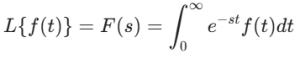
For this formula, s represents a complex frequency component. Function $f(t)$ is required to be both piecewise continuous and have exponential boundedness so that the resulting integral converges. This specific definition underpins subsequent sophisticated uses in Mathematical Physics methods and is vital for those studying for the RPSC Assistant Professor Physics Paper II. Grasping this integral enables the manipulation of intricate physical models featuring time-invariant coefficients.
Linearity and Shifting Properties of Laplace Transforms
Linearity grants the ability to spread the transformation across sums and multiples of functions. When dealing with a pair of functions and two constants, the transformation of their combined form is equivalent to the combined form of their separate transformations. This characteristic streamlines the examination of combined signals within physical setups. It confirms that intricate mathematical expressions can be separated into simpler, more workable components during computation.
To swiftly undertake exercises, you need to retain particular mappings for basic functions. he first shifting theorem states that if the transform of f(t) is F(s), then the transform of eatf(t) is F(s − a). These basic equations serve as the foundation for more complex topics in RPSC Assistant Professor Physics Paper II.
Essential Formulas for Common Functions
You must memorize specific transforms for elementary functions to solve problems quickly. For a constant function f(t) = 1, the transform is 1/s. For a power function f(t) = tn, the result involves the gamma function or factorials. Trigonometric functions like sine and cosine also have distinct algebraic representations in the s domain. These formulas are the building blocks for more advanced Mathematical Methods of Physics.
Numerical expressions of the theorem include:
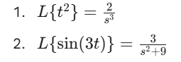
For the RPSC Assistant Professor Physics Paper II, swiftness and precision in using these equations are key to passing. Drilling these fundamental structures aids in spotting trends within more intricate inverse scenarios. These essential elements are crucial for any student tackling Mathematical Methods of Physics.
The Role of Inverse Laplace Transforms in Physics
Inverse Laplace Transforms retrieves the initial time-based function from its frequency spectrum representation. Whereas the forward operation streamlines the equation, the inverse operation yields the tangible result. This procedure frequently necessitates breaking down the expression using partial fractions to align the s-domain form with recognized basic templates. It constitutes a vital stage in determining the temporary behavior of electrical networks or physical vibrators.
The symbol for Inverse Laplace Transforms is L-1\F(s) = f(t). Mathematically, this involves a Bromwich integral in the complex plane, though most physics problems use lookup tables. For example, if you find a solution F(s) = 1/(s-4), then Inverse Laplace Transforms yield f(t) = e4t. Aspiring RPSC Assistant Professor Physics Paper II contenders need skill in these inverse processes to finalize problem resolution. Absent the capacity to shift back to the real domain, the conversion’s outcome stays theoretical and impractical.
Applications in RPSC Assistant Professor Physics Paper II
The RPSC Assistant Professor Physics Paper II syllabus requires a deep understanding of mathematical tools. Laplace Transforms appear frequently in sections dealing with classical mechanics, electromagnetism, and circuit theory. These transforms turn linear differential equations into algebraic equations, which you then solve for the unknown variable. This application is a cornerstone of Mathematical Methods of Physics used by successful candidates.
To get ready properly, you ought to group subjects based on how often they show up in the test documents. The table below shows how important mathematical and physics subjects are distributed for the RPSC Assistant Professor Physics examination.
| Exam Paper | Key Topics and Focus Areas |
|---|---|
| Paper I | Classical Mechanics, Quantum Mechanics, Mathematical Physics (Basic), Electrodynamics |
| Paper II | Thermodynamics, Statistical Physics, Atomic and Molecular Physics, Laplace Transforms, Nuclear Physics |
Concentrating on the distinct demands of Paper II allows for focused preparation. Employing organized charts like the preceding one aids in distributing study hours according to the significance of Inverse Laplace Transforms and related subjects.
Limitations and Critical Perspective on Transform Methods
Laplace Transforms prove useful, yet they don’t resolve every differential equation. This technique principally works for linear equations whose coefficients remain constant. Should a system exhibit nonlinearity or time-varying coefficients, the conventional transform method frequently falls short. For these scenarios, numerical techniques or alternative integral transforms, such as the Fourier or Mellin transforms, could be required.
A further restriction concerns the starting state. Laplace Transforms inherently account for the beginning state at t = 0. Should your physical situation demand limits at other locations, this approach turns unwieldy. One needs to discern when the Frobenius method or Green functions offer a superior fit. Grasping these limits stops one from utilizing an instrument in a situation where it proves inefficient or inapplicable.
Practical Scenario: Solving a Damped Harmonic Oscillator
Think about a weight attached to a spring that has damping, a standard scenario in Mathematical Methods for Physics. Its motion is governed by a second-order differential equation. By using Laplace Transforms on every part, you substitute derivatives with powers of ‘s’. This transformation lets you find the position function X(s) through straightforward algebraic manipulation. This concrete example shows how conceptual mathematics tackles tangible physical movement.
Once you have the expression for X(s), you use Inverse Laplace Transforms to find x(t). If the system is underdamped, the inverse result will show a decaying sine wave. This outcome matches physical observations of a vibrating spring losing energy. For students of RPSC Assistant Professor Physics Paper II, mastering this specific scenario is vital. It links theoretical transforms to observable physical phenomena, reinforcing the utility of the math.
Conclusion
Exploring Laplace Transforms transcends just a mathematical drill; it’s an essential competency for any dedicated physicist. This approach offers a structured link connecting how things behave over time with their frequency spectrum analysis, converting overwhelming differential equations into solvable algebraic tasks. Although the method has boundaries, notably concerning non-linear systems, its effectiveness in resolving linear issues along with starting values remains superior.
Grasping these changes provides a clearer lens to view physical setups than typical calculus methods usually allow. VedPrep furnishes thorough instruction and skilled materials to aid your command of these mathematical approaches for the RPSC Assistant Professor test. Steady rehearsal involving both primary and reverse procedures will guarantee preparedness for the toughest analytical hurdles in your scholarly pursuits.
To know more in detail from our faculty, watch our YouTube video:
Frequently Asked Questions (FAQs)
Why are Laplace Transforms used in Physics?
Physicists use these transforms to analyze linear time invariant systems. They simplify the calculation of transient responses in circuits and mechanical oscillators. The method handles initial conditions naturally within the transformation process. This makes it a primary tool in Mathematical Methods of Physics.
What is the range of integration for a Laplace Transform?
The standard unilateral Laplace Transform integrates the function from zero to positive infinity. You multiply the function by an exponential decay term before integrating. This range ensures the transform captures all system behavior starting from a specific initial time.
What is the s variable in Laplace Transforms?
The variable s represents a complex frequency parameter. It consists of a real part and an imaginary part. This complex variable allows the transform to map stability and frequency characteristics of a physical system. It serves as the foundation for frequency domain analysis.
How do you calculate Inverse Laplace Transforms?
You find the original time domain function by reversing the transformation. Most practitioners use lookup tables of standard pairs. If the expression is complex, you apply partial fraction decomposition to break it into recognizable terms. This step is vital for RPSC Assistant Professor exam problems.
What is the Linearity Property in Laplace Transforms?
The linearity property states that the transform of a sum equals the sum of individual transforms. You can also pull constant coefficients out of the integral. This allows you to process complex signals by breaking them into simpler components. It streamlines calculations in Mathematical Methods of Physics.
How does the First Shifting Theorem work?
This theorem describes how multiplying a function by an exponential in time results in a shift in the s domain. If you know the transform of a function, you can find the transform of its exponentially scaled version. It helps solve equations involving damped oscillations.
Why might a Laplace Transform fail to converge?
A transform fails to converge if the function grows faster than the exponential decay term. Functions with vertical asymptotes or certain types of rapid growth do not have a defined transform. You must ensure the function is of exponential order for the method to apply.
What happens if the s variable is outside the Region of Convergence?
If the s variable does not fall within the Region of Convergence, the integral does not result in a finite value. Every transform has a specific range of s where it is valid. Using values outside this range leads to incorrect physical interpretations and mathematical errors.
How do you fix errors in partial fraction expansion?
Most errors occur during the determination of coefficients. You should verify your results by substituting values of s or finding a common denominator to return to the original form. Double checking these constants is essential for accuracy in the RPSC Assistant Professor exam.
What are the Laplace Transforms of periodic functions?
You can find the transform of a periodic function by integrating over a single period and dividing by a specific exponential factor. This allows you to analyze repeated waveforms like square or sawtooth waves. It is a common topic in advanced Mathematical Methods of Physics.
How does the Convolution Theorem simplify problems?
The convolution of two functions in the time domain corresponds to the simple multiplication of their transforms. This theorem is useful when finding the output of a system given an arbitrary input. It avoids the need for complex time domain convolution integrals.
What is the transform of the Dirac Delta function?
The Laplace Transform of a unit impulse at time zero is exactly one. This result makes the Dirac Delta function a powerful tool for finding the transfer function of a physical system. It represents the system response to an instantaneous force.
How do you transform an integral of a function?
The transform of the integral of a function is the transform of the function divided by s. This property is useful for solving integro differential equations found in circuit analysis. It further demonstrates how the s domain simplifies calculus operations.
What is the Final Value Theorem?
The Final Value Theorem allows you to find the steady state value of a function as time approaches infinity. You calculate the limit of s multiplied by the transform as s approaches zero. This provides quick insights into system stability without a full inverse transform.